Control Room

Fig.1 SRT control room layout.

ACS Command Center

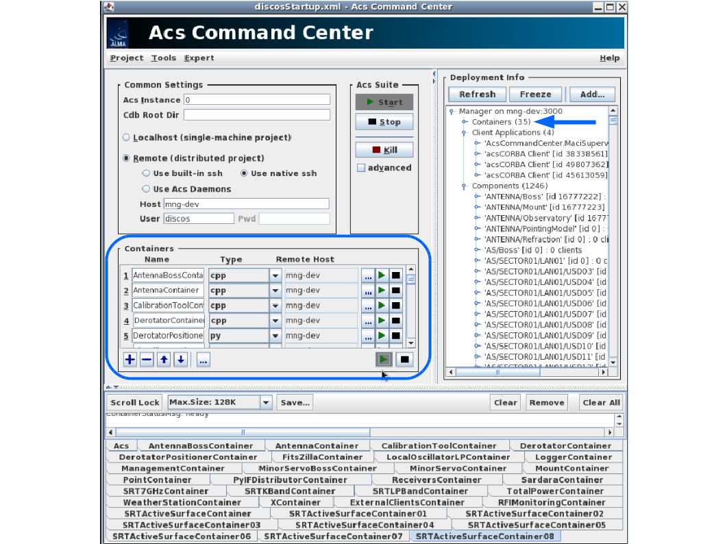
Fig.2 The ACS monitor shows the state of the containers related to each DISCOS component. The state of each container can be verified in the section highlighted in blue. The blue arrow indicates the number of containers (35 when the system is ready).

ACS Command Center

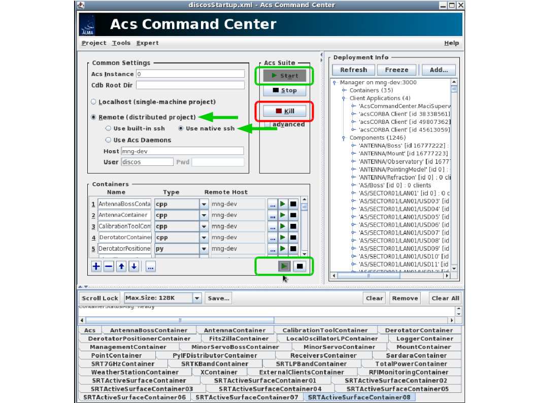
Fig.3 In the Common settings panel of the ACS monitor, the remote and the use native ssh items must be selected as indicated by the green arrows. The Start and the global green triangle buttons highlighted in green must be used to restart the Acs suite and the Containers, respectively. The Kill button highlighted in red must be used to close the ACS panel during the Shutdown of Discos.

Active Surface

Fig.4 This monitor shows the status of the actuators in a graphical representation of the Active Surface and its configuration.

Active Surface

Fig.5 After parking the active surface by using > asPark, in the Active Surface monitor the status of the Actual Profile box is Park.

Active Surface

Fig.6 The Active Surface monitor in the parabolic configuration.

Active Surface

Fig.7 The status of the active surface is WARNING after the “Restart Discos” procedure.

Logging Display

Fig.8 The Logging Display shows the log messages related to the observation. New messages are shown over the previous ones.

Meteo Client

Fig.9 The Meteo Client window shows the atmospheric temperature and wind parameters (including wind direction) using a graphic interface.

Discos-console

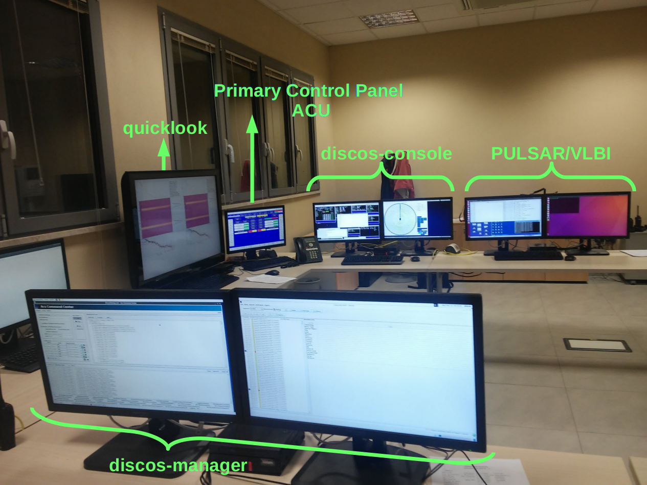
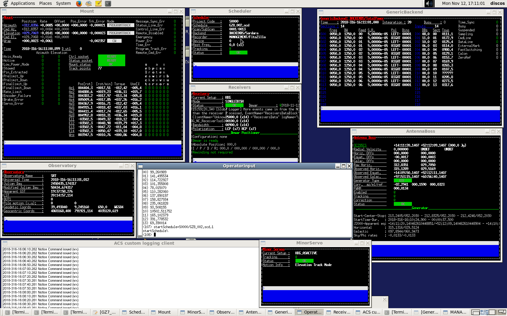
Fig.10 Discos-console is the machine where you run the system and where you should find the input terminal and all the monitors. It is also the destination for your schedules.

OperatorInput

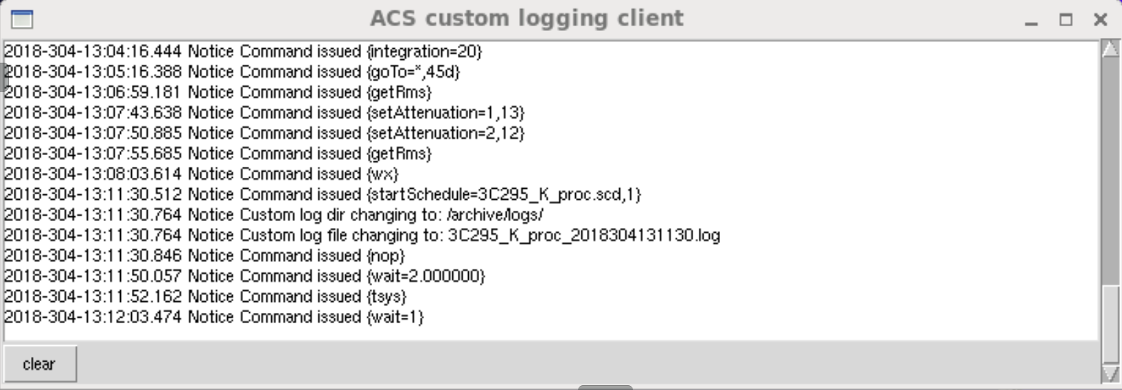
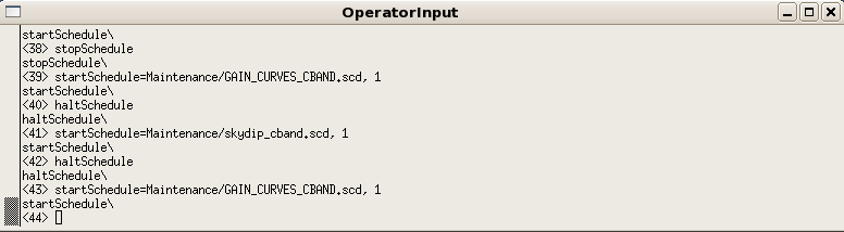
Fig.11 In the input console the users can write Nuraghe commands. The prompt is just a sequential number enclosed in <>. If a command is properly read, the system replies by repeating the command itself, followed by the operation results (if they are foreseen).

AntennaBoss

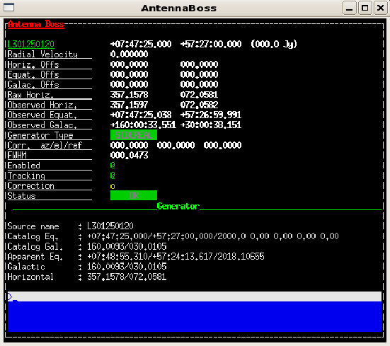
Fig.12 The AntennaBoss monitor shows the target info, indicating the commanded and actual positions pointed by the antenna. It also gives a feedback on the pointing accuracy and on the overall antenna status.

GenericBackend

Fig.13 The monitor GenericBackend shows the backend setup parameters related to each section.

Fig.14 The monitor GenericBackend in the K-band configuration.

Mount

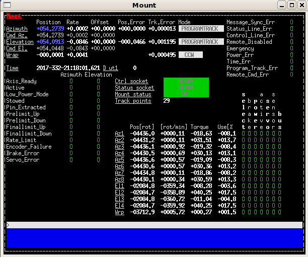
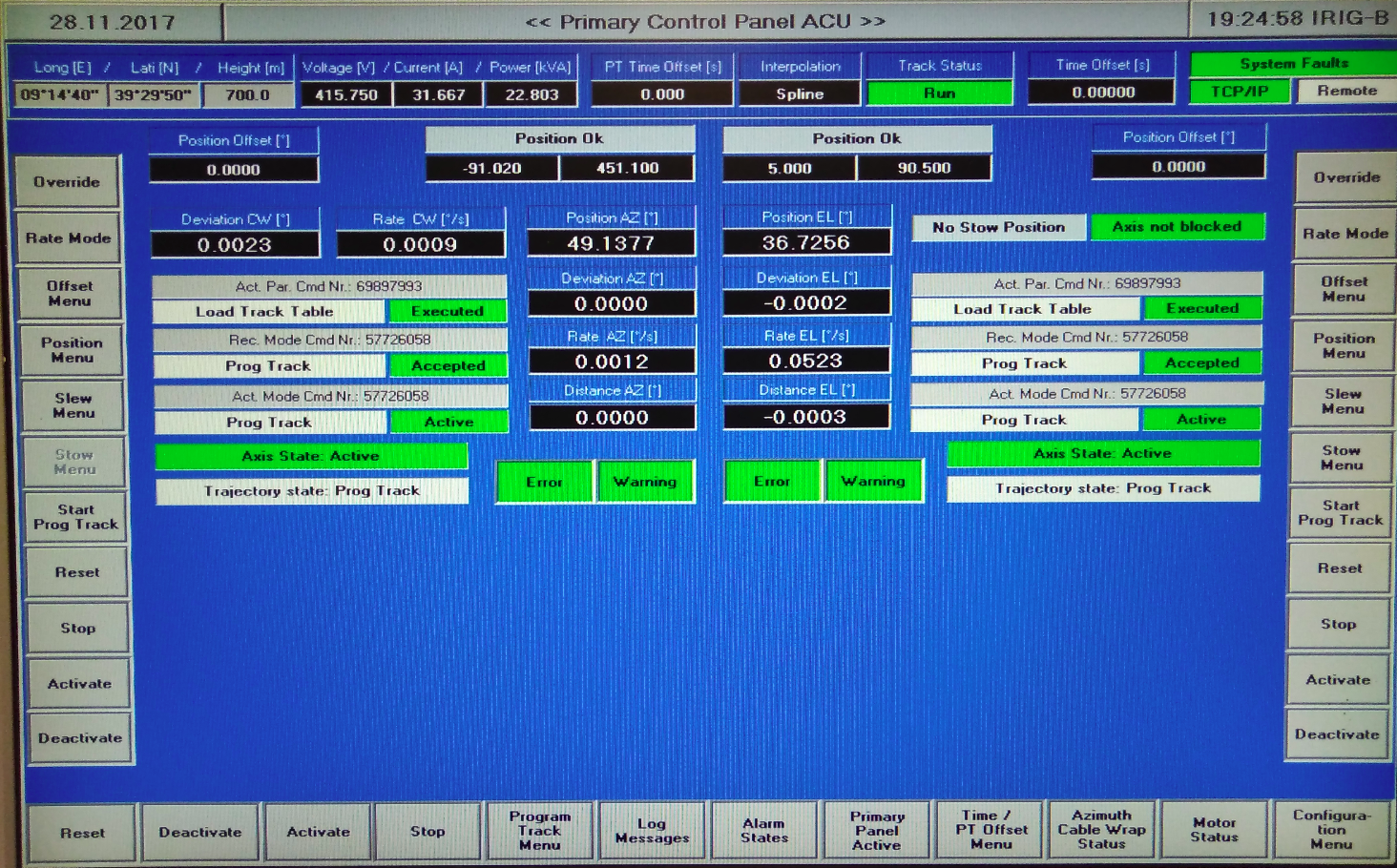
Fig.15 Observers need to focus only on the Mount status (indicated by the green box) and on the actual position of the axis expressed in Azimuth and Elevation (shown in blue), compared to the commanded positions (actual positions with the label “Cmd Az.” and “Cmd El.”).

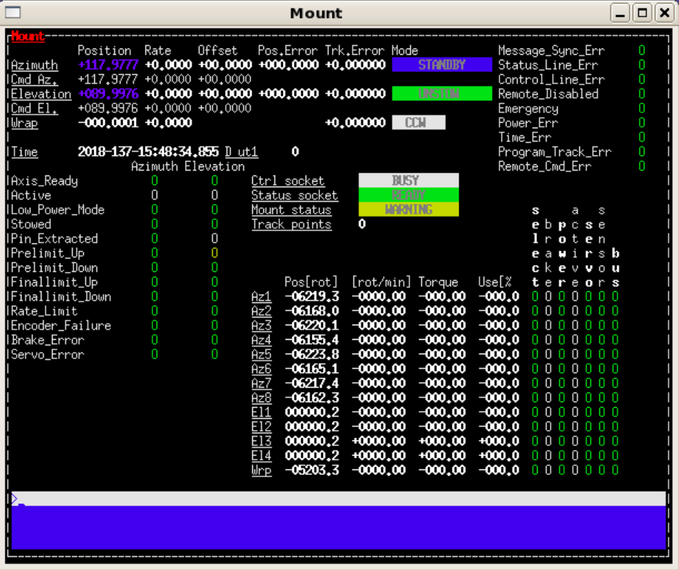
Fig.16 The Mount monitor after the park of the antenna by using > antennaPark

Observatory

Fig.17 The Observatory monitor shows the station time and coordinates.

ReceiversBoss

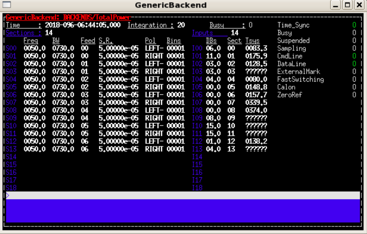
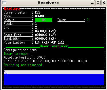
Fig.18 The ReceiverBoss monitor summarizes the frontend setup parameters. The bottom part is devoted to the derotator (dewar positioner), when available.

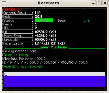
Fig.19 The ReceiverBoss monitor in the L-band configuration.

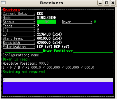
Fig.20 The ReceiverBoss monitor in the K-band configuration.

Scheduler

Fig.21 The Scheduler monitor shows the details on the selected data acquisition devices and on the running schedule, if any.

Fig.22 The Scheduler monitor after the interruption of the current subscan by using > stopSchedule or > haltSchedule

MinorServo

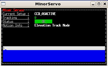
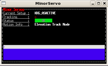
Fig.23 The MinorServo monitor shows the current setup code and the minor-servo status and movement. In this case the image refers to the C-band configuration.

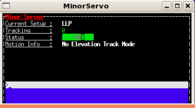
Fig.24 The MinorServo monitor in the L-band configuration.

Fig.25 The MinorServo monitor in the K-band configuration.

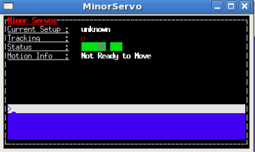
Fig.26 The MinorServo monitor after the park of the minor servos by using > servoPark

Calibration tool client

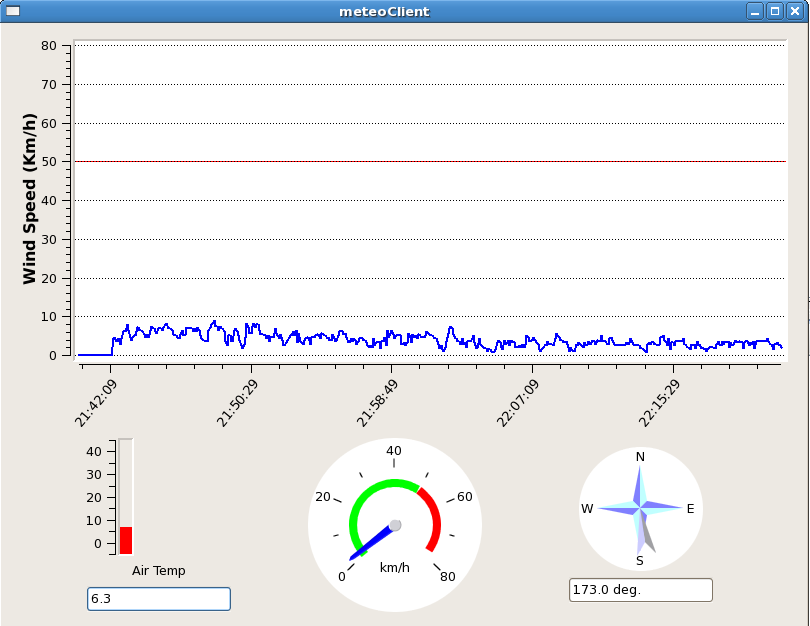
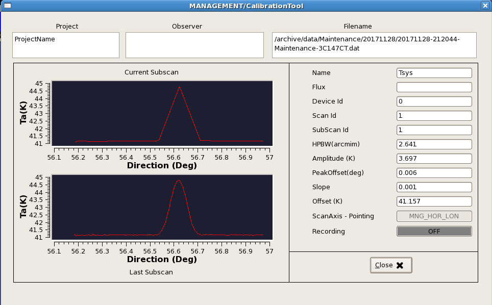
Fig.27 In the Calibration tool client window the subscan currently being acquired is shown in real-time (upper plot), even if in a low-resoltution. In the lower plot, the last completed subscan - in its full sampling - is shown. We can read the information about the pointing of focus offsets (“peakoffsets”), the beam size (“HPBW”), etc.

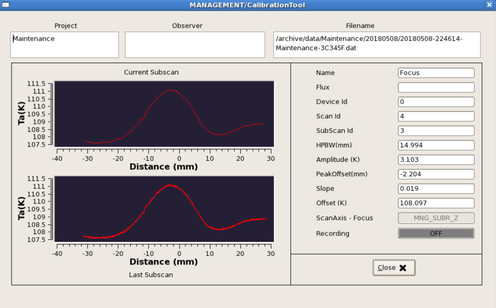
Fig.28 Calibration tool client window related to a focus subscan.

GenericBackendX

Fig.29 A second GenericBackend panel shows the setup parameters of each section of Xarcos.

Primary Control Panel ACU

Fig.30 Primary Control Panel ACU.

SEADAS

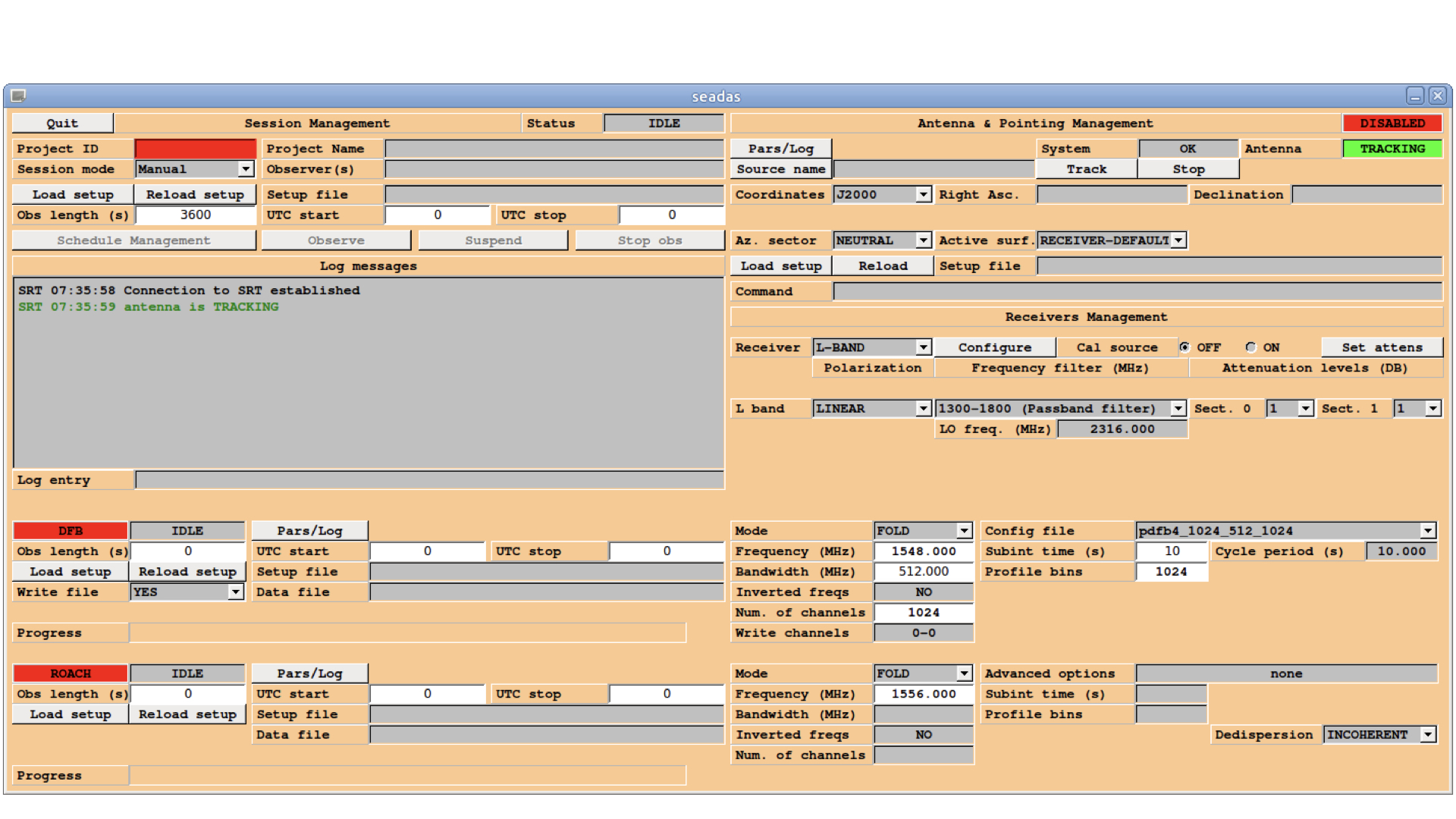
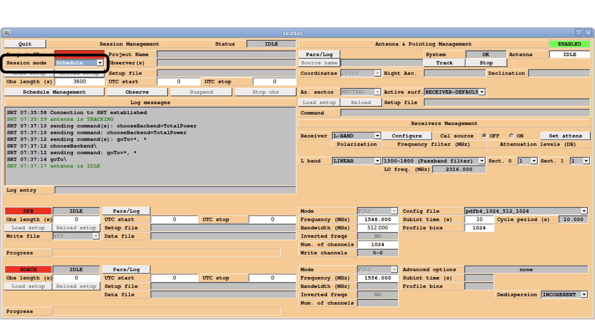
Fig.31 Seadas GUI. On the top right, the red box signals that the control of the antenna is DISABLED.

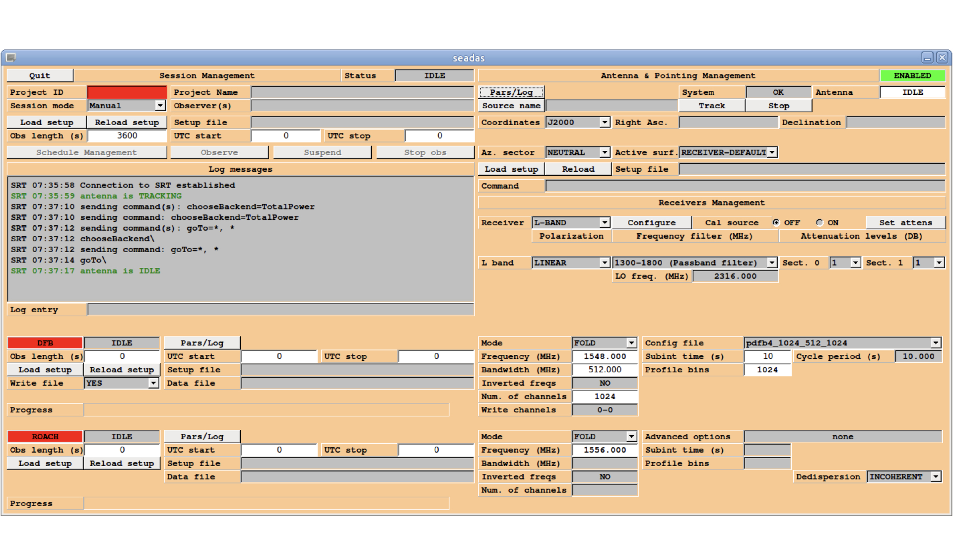
Fig.32 Seadas GUI. On the top right, the green box signals that the control of the antenna is now ENABLED.

Fig.33 Seadas GUI. On the top left, circled in black, the Session Mode combo box where the option Schedule needs to be selected in order to start the observations through your pre-prepared schedule.

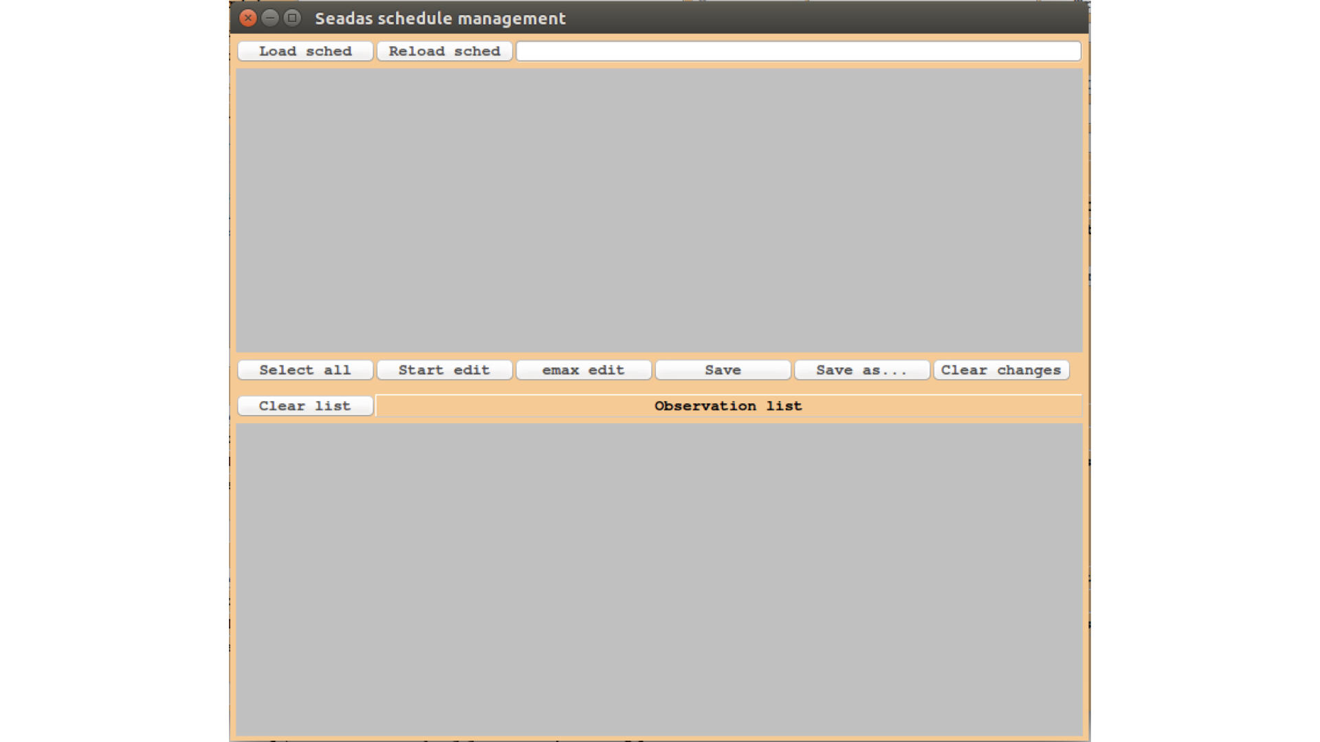
Fig.34 Seadas GUI. Pop-up window where the schedule can be uploaded by clicking on the button Load sched.

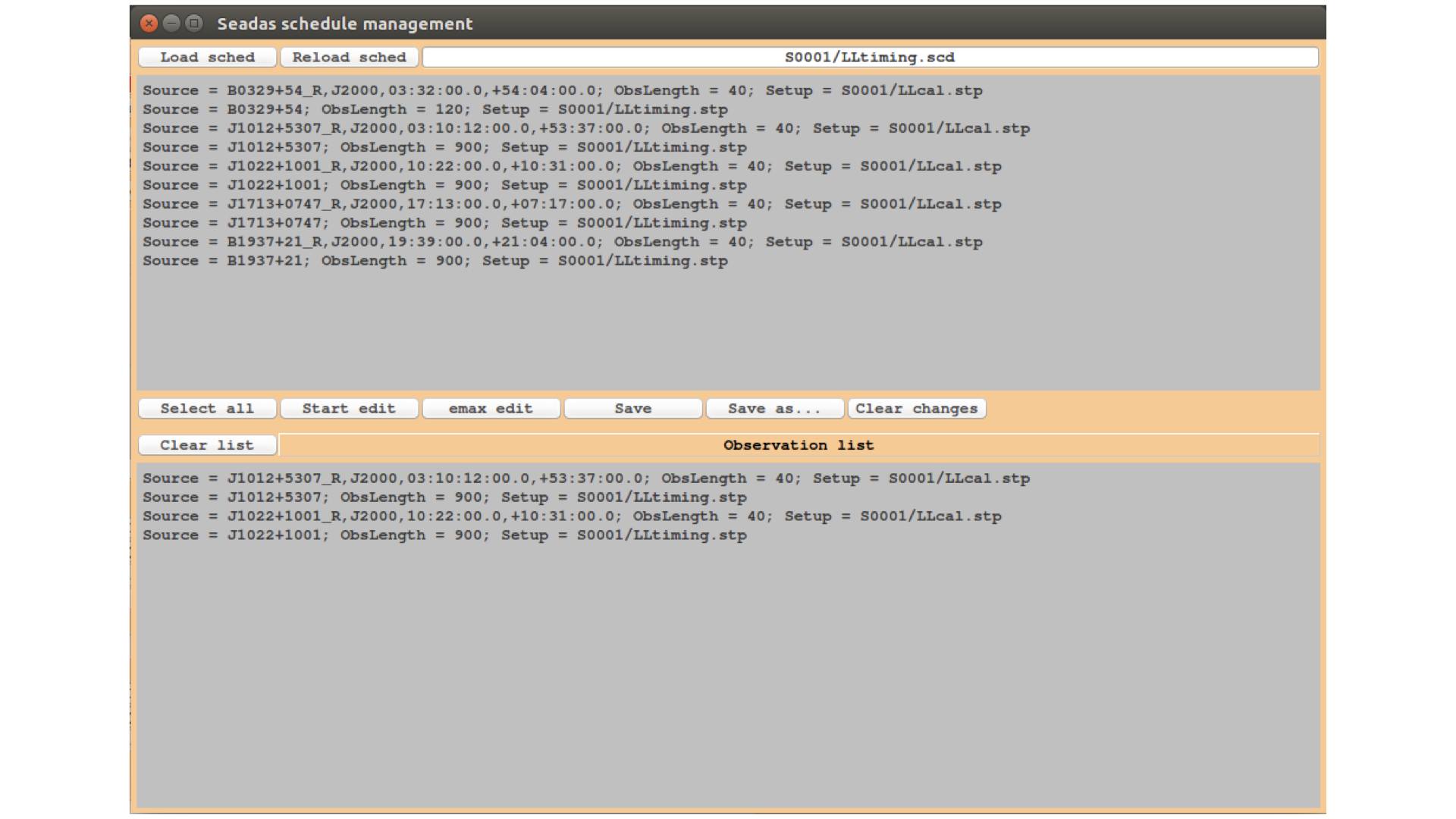
Fig.35 Seadas GUI pop-up window for schedule management. The uploaded schedule lines will appear on the top panel. The ones selected for observations will appear in the bottom panel.